
How to Create an Instrument Method in Empower
This guide walks you through how to create an instrument method in Empower using the Instrument Method Editor and its built-in wizard. You will learn how to log on, select your project and system, configure the pump gradient, sampler, column compartment, and UV detector settings, and save your finished method for use in sample runs.
Video: SII User Experience for Waters Empower 3: Creating instrument methods for a Thermo Scientific UHPLC by Chromatography & Mass Spectrometry Solutions (2019). All credit for the demonstration goes to the creator; watch the original on YouTube. The written guide below was generated from this video by Docsie. Creator? Request a change or removal.
This guide walks you through how to create an instrument method in Empower using the Instrument Method Editor and its built-in wizard. You will learn how to log on, select your project and system, configure the pump gradient, sampler, column compartment, and UV detector settings, and save your finished method for use in sample runs.
Prerequisites
- Access to the Empower 3 software with a valid user name and password.
- A chromatographic system (for example, a Vanquish Horizon system) configured and available in Empower.
- A project set up in Empower in which to acquire data.
Log on to Empower 3
Locate and open the Empower 3 application on the Windows desktop. When the login dialog appears, enter your user name and password in the respective fields, then click OK. The login window appears centered on screen, with the instruction "Log on with your user name and password" shown at the bottom.
Select your project and system
Once you are logged in, the Run Samples window opens. In the Project in which to acquire data section, select your project from the list (for example, "SII for Empower Test"). In the Chromatographic Systems section, select the appropriate system (for example, "Vanquish_Horizon"), then click OK to confirm your selections.
Open the Instrument Method Editor
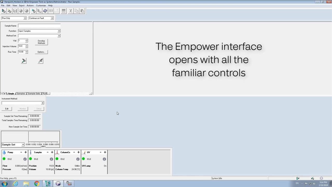
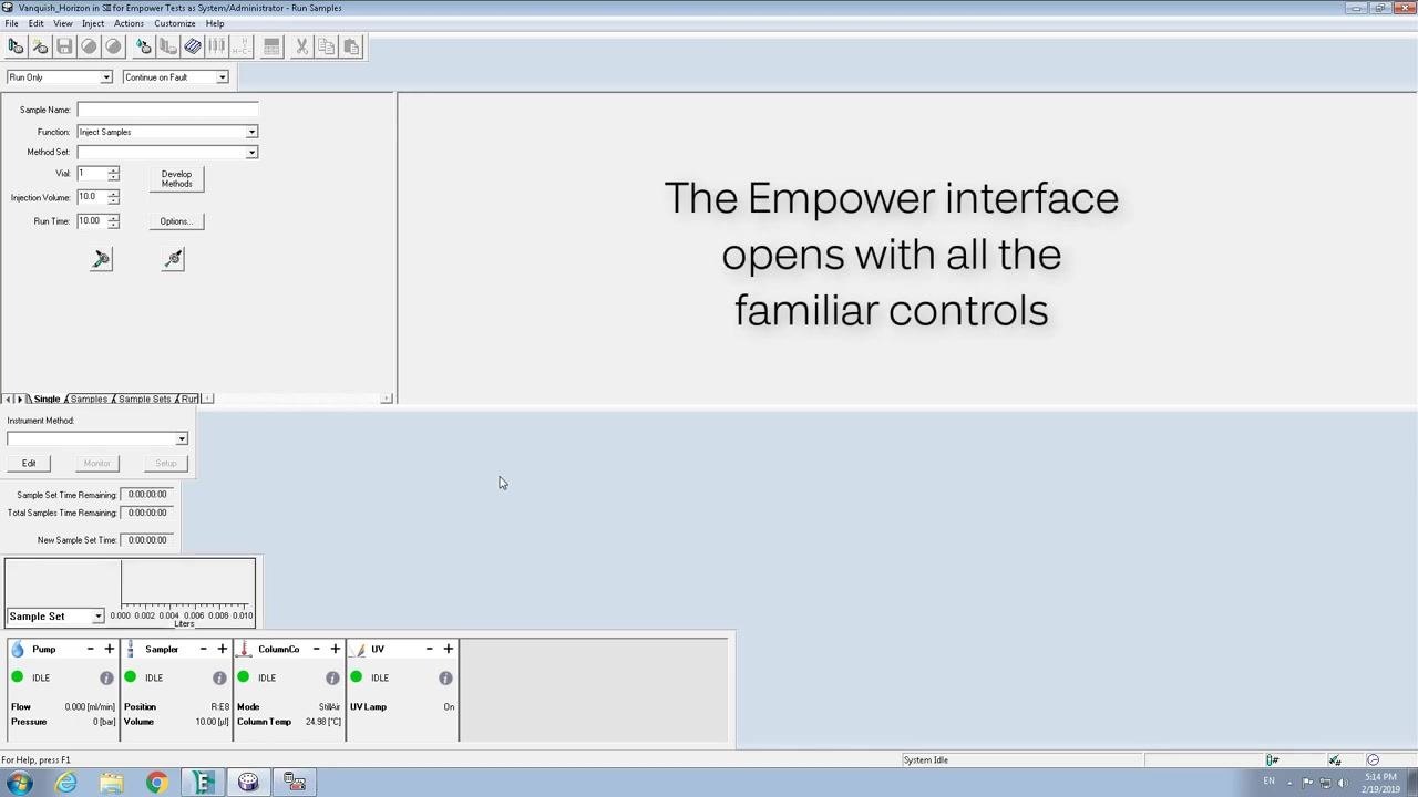
The Empower interface opens with all familiar controls and panels. The main window shows fields for sample name, function, method set, injection volume, and run time, along with instrument method controls. The lower section lists the status of each system module (Pump, Sampler, Column Compartment, UV, and so on), all showing "IDLE" status.
In the Instrument Method section, click Edit to open the Instrument Method Editor. The editor opens on the General Settings for System tab. Enter the desired run time in the Run Time field (for example, 20.000 min). Under Diagnostic Channels, select the channels you want to use (for example, "ICC_Temp," "PCC_Temp," "Pump_Pressure"), using the Select all channels or Deselect all channels buttons as needed. The Thermo Scientific Program Wizard guides you through the rest of the method setup.
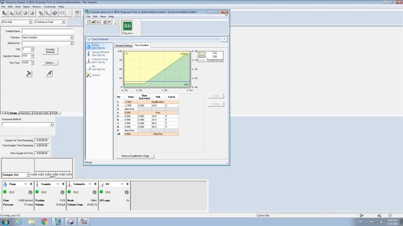
The left panel of the editor displays an icon for each module: Pump (VH-P10-A), SampleModule (CH-1A1-A), ColumnComp (VH-D10-A), UV (VH-D10-A), and System. Click any module icon to access and edit its specific settings. The main panel shows the Flow Gradient tab, with a graphical plot and gradient table displaying all programmed steps.
Configure the flow gradient for the pump
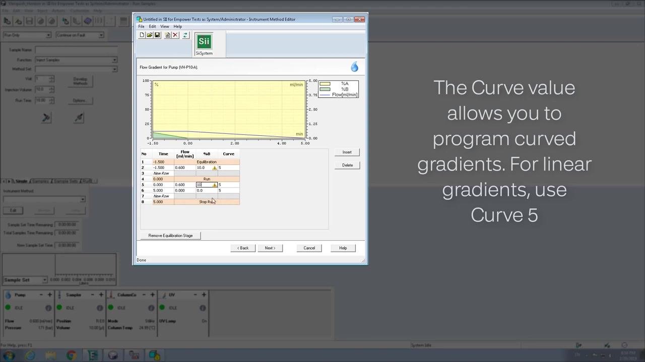
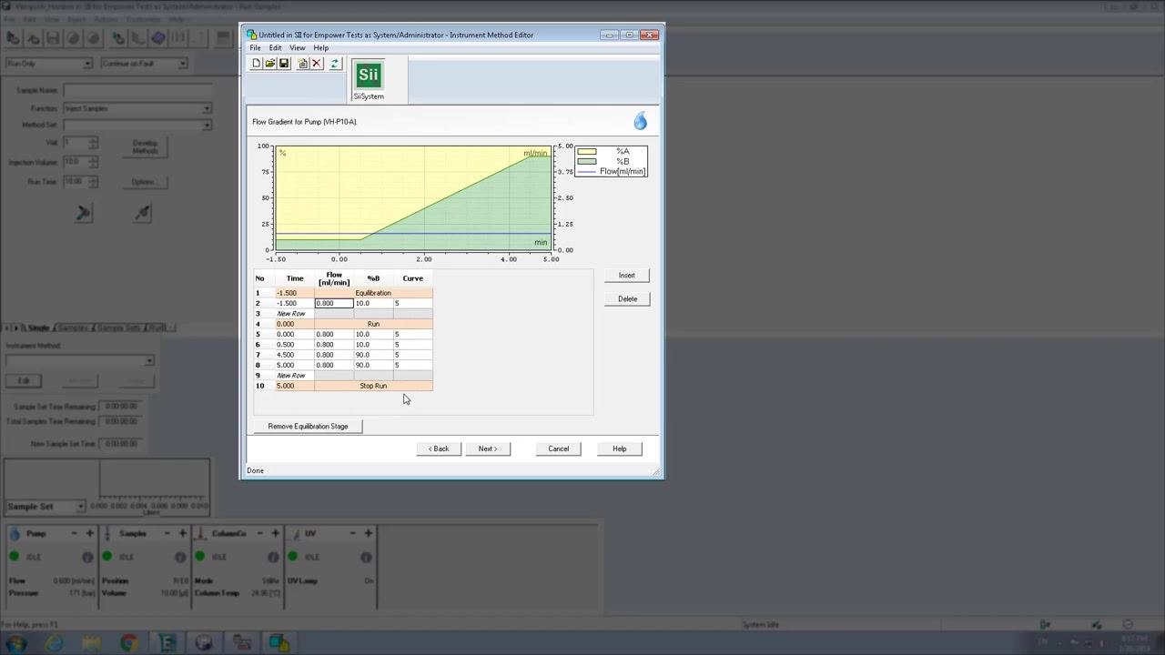
The Curve value lets you program curved gradients; for a linear gradient, set the Curve column to 5 for all steps. The gradient table lists steps for Equilibration, Run, and Stop Run, each with time, flow (mL/min), %B, and curve values. The plot above the table shows the gradient you have programmed.
Enter each gradient step to match your method requirements. A finalized table might look like this:
- -1.500 min: Flow = 0.800 mL/min, %B = 10.0, Curve = 5 (Equilibration)
- 0.000 min: Flow = 0.800 mL/min, %B = 10.0, Curve = 5 (Run)
- 0.500 min: Flow = 0.800 mL/min, %B = 10.0, Curve = 5 (Run)
- 1.000 min: Flow = 0.800 mL/min, %B = 90.0, Curve = 5 (Run)
- 5.000 min: Flow = 0.800 mL/min, %B = 90.0, Curve = 5 (Stop Run)
Click Next to continue to the next configuration step.
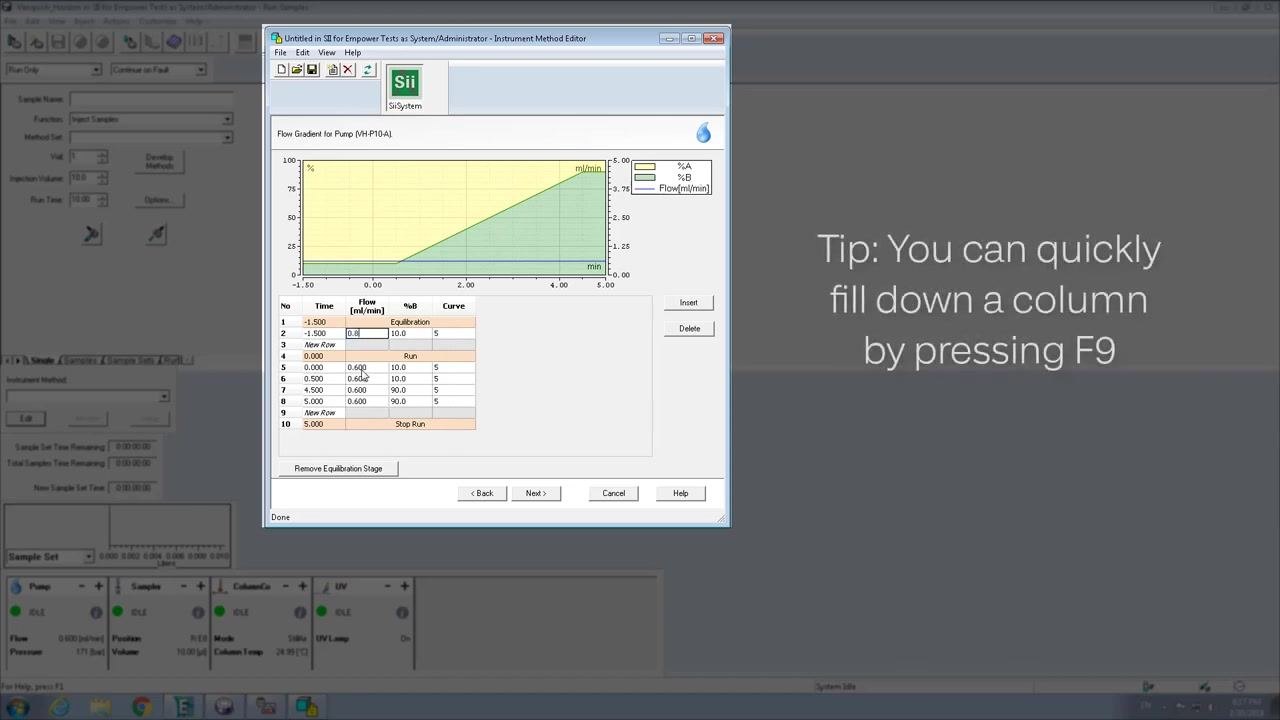
To speed up data entry, select a cell in the column you want to fill down and press F9 to copy that value into all rows below it. This shortcut is especially useful when you need the same flow rate or curve value across multiple steps.
Configure the sample module
In the General Settings for SampleModule window, set the draw and dispense speeds according to your sample viscosity and wash requirements:
- Draw speed: 20 (range 0.050–20.000 µL/s)
- Dispense speed: 5,000 (range 0.050–15,000 µL/s)
- Wash mode: NoWash
- Wash time: 2.0 s (range 0.0–300.0 s)
- Wash speed: 83.3 µL/s (range 10.0–83.3 µL/s)
Also set the connected pump and sample puncture offset if your method requires it.
The wizard always displays the valid range for each parameter, helping you avoid invalid entries. For example:
- Draw speed: 20 (range 0.050–20.000 µL/s)
- Dispense speed: 2 (range 0.050–15.000 µL/s)
- Wash mode: AfterDraw
- Wash time: 2.0 s (range 0.0–300.0 s)
- Wash speed: 83.3 µL/s (range 10.0–83.3 µL/s)
- Flow is delivered from: Pump
- Puncture offset: 0 (range 0.0–3,000 µm)
Adjust these values as needed for your method.
Set the column compartment temperature
In the Temperature Settings for ColumnComp window, configure the column and post-column cooler temperatures:
- Use temperature control for Column Chamber (CC): checked, Temperature 25.00°C (range 5.00–120.00°C), Thermostatting mode StillAir
- Use temperature control for Post Column Cooler (PCC): checked, Temperature 40.00°C (range 40.00–80.00°C)
Select Easy or Advanced mode depending on how much control you need, then click Next to continue.
Select the active column
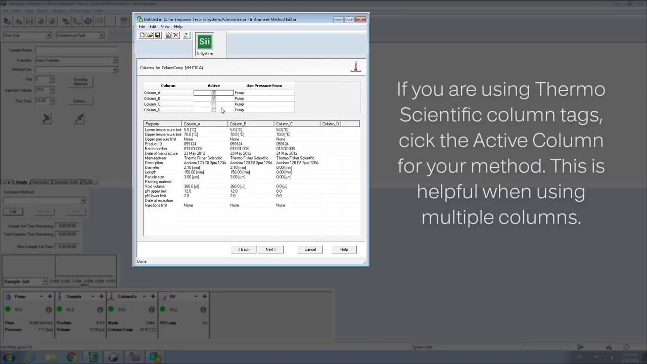
In the Columns for ColumnComp window, check the Active box for the column(s) you want to use with this method. Each column slot (A, B, C, D) displays its properties, including lower and upper temperature limits, upper pressure limit, product ID, batch number, manufacturer, date of manufacture, dimensions, packing material, void volume, pH limits, date of expiration, and injection limit.
If you use Thermo Scientific column tags, click the active column for your method; this is especially helpful when working with multiple columns. Click Next to proceed once the correct column is active.
Configure UV channel settings
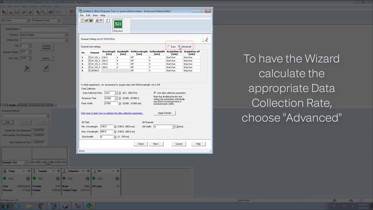
In the Channel Settings for UV window, select Advanced mode so the wizard can calculate the appropriate data collection rate. Configure each channel's wavelength, bandwidth, reference wavelength, and acquisition timing. For example:
- UV_VIS_1: 230.0 nm, Bandwidth 4 nm, RefWavelength Off, RefBandwidth 4 nm, Acquisition Start/Stop Run
- UV_VIS_2: 254.0 nm, Bandwidth 4 nm, RefWavelength Off, RefBandwidth 4 nm, Acquisition Start/Stop Run
- UV_VIS_3: 270.0 nm, Bandwidth 4 nm, RefWavelength Off, RefBandwidth 4 nm, Acquisition Start/Stop Run
- UV_VIS_4: 300.0 nm, Bandwidth 4 nm, RefWavelength Off, RefBandwidth 4 nm, Acquisition Start/Stop Run
- 3D FIELD: Off
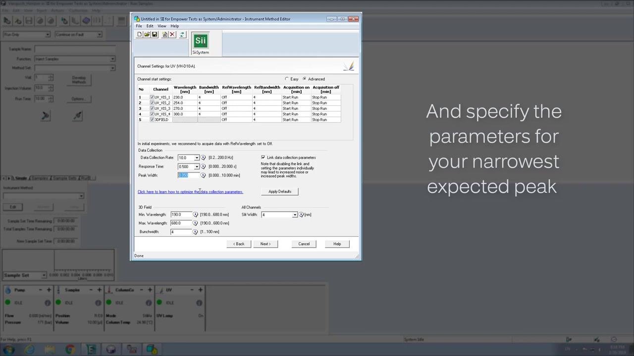
Set the Data Collection Rate (for example, 10.0 Hz), Response Time (for example, 0.500 s), and Peak Width (for example, 0.050 min), and configure the 3D Field and All Channels parameters as needed. Click Next to continue.
Specify parameters for your narrowest expected peak
Still in the Channel Settings for UV window, set the data collection parameters to match your narrowest expected peak:
- Data Collection Rate: 10.0 Hz (range 0.2–200.0 Hz)
- Response Time: 0.500 s (range 0.020–20.000 s)
- Peak Width: 0.050 min (range 0.010–10.000 min)
Check Link data collection parameters if you want these settings synchronized across all channels. Adjust the 3D Field and All Channels parameters as needed:
- Min. Wavelength: 190.0 nm
- Max. Wavelength: 680.0 nm
- Slit Width: 4 nm
- Bunchwidth: 4 (range 1–100 nm)
Use Apply Defaults at any time to revert to recommended settings, and consult the help link for guidance on optimizing data collection parameters.
Save and name your method file
With all settings finalized in the Instrument Method Editor, use the save functionality (typically available from the File menu or the save icon) to store your method under a descriptive name. Confirm that the method now appears in your method list for future selection.
Find and select your new method
Return to the Empower home page or the main Run Samples screen. Your newly created method is now available there. In the Instrument Method dropdown, select your new method (for example, "5 minute quick run").
Set up the system for sample runs
With your method selected, click Setup to configure the system for sample analysis. Confirm that all modules (Pump, Sample, ColumnComp, UV) show the "IDLE" state and that the method parameters are correctly loaded and displayed.
What's next
Your instrument method is now saved and ready for use. You can select it from the Instrument Method dropdown whenever you set up a new sample run, and continue configuring your sample set and acquisition parameters as required for your analysis.
Generation details: cost, quality tiers
Docsie billed 2,500 credits ($1.75) to analyze this 5-minute video at standard quality. The rewrite, template fill and Word/PDF exports were included. The same video at each quality tier:
| Quality | Frames sampled | Credits | Approx. cost |
|---|---|---|---|
| Draft | every 16-30 s | 1,250 | $0.88 |
| Standard (this guide) | every 8-15 s | 2,500 | $1.75 |
| Detailed | every 4-7 s | 5,000 | $3.50 |
| Ultra | every 1-3 s | 10,000 | $7.00 |
Credits priced at $0.70 per 1,000; plans include a monthly allowance. Enterprise customers on on-premise or bring-your-own-model deployments run this on their own inference and pay no per-video credits.
Generated by Docsie Video-to-Docs on 2026-10-11 from a 4-minute video. Screenshots are frames from the source video and belong to their creator, Chromatography & Mass Spectrometry Solutions, whose original is embedded above. If you own this video and want the guide removed or credited differently, contact us and we will act within one business day.